Linear Programming

Linear Programming is a particular case of constrained optimization problems. What sets the linear programming aside is that optimal values are sought for a linear function subject to linear constraints. To have a general formulation let's assume that we are given

  1. an m×n matrix A
  2. an m×1 (column) vector b
  3. a 1×n (row) vector c

The role of the unknown is played by a n×1 (column) vector x which is required to satisfy two constraints:

  1. Ax = b, and
  2. x0,

the latter means that all the components of x are nonnegative. Vectors that satisfy constraints 1 and 2 are called feasible. We are interested in the situations where the set of feasible vectors is not empty.

Finally, the cost or objective function f is given by f(x) = c·x, where c·x is the scalar product of two vectors c and x: c·x = c1x1 + ... + cnxn. In linear programming, one is requested to maximize (or minimize) the cost function f subject to constraints 1 and 2:

(P) Maximize f(x) = c·x subject to Ax = b and x0

Example

Assume that we have decided to position defenders of a square castle according to the following plan:

(*)
pqp
q0q
pqp

so that the total number of defenders is 4(p + q) while (2p + q) fighters face the enemy on every side. Let's denote p = x1 and q = x2. Let also A = (4 4), be a 1×2 matrix, and c = (2 1), a 1×2 row vector. Assume that a 1×1 vector b is equal to (28). The linear programming problem (P) is then interpreted as:

How to position 28 fighters according to the symmetric arrangement above so as to have the maximum number of defenders on each side?

In a more formal manner, the problem is to maximize f(x) = 2x1 + x2 subject to 4(x1 + x2) = 28 and x1 ≥ 0 and x2 ≥ 0. Geometrical solution to the problem is easy and illuminating. 
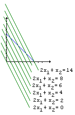
The set F of feasible vectors is defined by

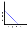
  F = {x: x1 + x2 = 7 and x1 ≥ 0 and x2 ≥ 0}.

In the plane with orthogonal axes x1 and x2, F is a straight line segment between two points: (0, 7) and (7, 0).

The function f depends on two variables: x1 and x2. Instead of drawing its graph in the three-dimensional space, we'll draw a series of its level lines in the plane. The function is constant on each of the lines as shown on the diagram at the left. The function attains the maximum value 14 on the line 2x1 + x2 = 14 that passes through one of the endpoints (7, 0) of the interval F. This is always the case in linear programming problems - solution is found at one (or more) vertices of the set of feasible vectors. Note that if we were looking to minimize f the solution would be located at the other endpoint (0, 7) of F. Thus for the arrangement (*) we have two extreme configurations: a minimum and a maximum:

 
070
707
070
707
000
707

References

  1. J. L. Casti, Five Golden Rules, John Wiley & Sons, 1996
  2. J. A. Paulos, Beyond Numeracy, Vintage Books, 1992
  3. G. Strang, Introduction to Applied Mathematics, Wellesley-Cambridge Press, MA, 1986.

Related material
Read more...

A Sample of Optimization Problems

  • Mathematicians Like to Optimize
  • Reshuffling knights - castle defenders
  • Isoperimetric Theorem and Inequality
  • Viewing a Statue: the Problem of Regiomontanus
  • Fagnano's Problem
  • Minimax Principle Demonstration
  • Maximum Perimeter Property of the Incircle
  • Extremal Problem in a Circular Segment
  • Optimization in Four Variables with Two Constraints
  • Daniel Dan's Optimization in Three Variables
  • Problem in a Special Trapezoid
  • Cubic Optimization with Linear Constraints
  • Cubic Optimization with Partly Linear Constraints
  • Problem M317 from Crux Mathematicorum
  • Find the Maximum and Minimum of a Function
  • Area of Isosceles Triangle
  • Minimum of Cotangents from Saint Petersburg

  • |Contact| |Front page| |Contents| |Algebra| |Up|

    Copyright © 1996-2018 Alexander Bogomolny

    71550934