Inflection Points of Fourth Degree Polynomials

In an article published in the NCTM's online magazine, I came across a curious property of 4^th degree polynomials that, although simple, well may be a novel discovery by the article's authors (but see also another article.) Their research began with a suggestion for investigation of the inflection points of 4^th degree polynomials from a 2002 issue of Mathematics Teacher, another NCTM publication.

A fourth degree polynomial will be written as

p(x) = m₄x⁴ + m₃x³ + m₂x² + m₁x + m₀.

In the applet and text below, I shall describe the polynomials by their coefficients, with the exponent of x and the index of its coefficient on the left, like this:

4: m₄

3: m₃

2: m₂

1: m₁

0: m₀

4^th degree polynomials may or may not have inflection points. These are the points where the convex and concave (some say "concave down" and "concave up") parts of a graph abut. The second derivative of a (twice differentiable) function is negative wherever the graph of the function is convex and positive wherever it's concave. The second derivative is 0 at the inflection points, naturally.

If a 4^th degree polynomial p does have inflection points a and b, a < b, and a straight line is drawn through (a, p(a)) and (b, p(b)), the line will meet the graph of the polynomial in two other points. Let's denote their abscissas x_L and x_R assuming

x_L < a < b < x_R.

Solving equations involving second derivatives of 4^th degree polynomials may tax one's desire to see a problem through. Authors McMullin and Weeks used an ingenious device of not solving the equation at all. Instead, knowing that a and b satisfy a quadratic equation, they wrote the equation (p''(x) = 0) in the form

p''(x) = 12m₄(x - a)(x - b).

The polynomial p(x) can now be expressed from p''(x) by repeated integration:

4: m₄

3: -2(a + b)m₄

2: 6abm₄

1: m₁

0: m₀

Writing an equation of the line L(x) through (a, p(a)) and (b, p(b)) is straightforward. (In the applet, the line is referred to as the "inflection line."). The difference p(x) - L(x) is a 4^th degree polynomial with coefficients

(*)

4:		m₄
3:		-2(a + b)m₄
2:		6abm₄
1:		(a³ - 3a²b - 3ab² + b³)m₄
0:		-ab(a² - 3ab + b²)m₄

Along with a and b, x_L and x_R, are the solutions of

p(x) - L(x) = 0.

At this point, McMullin and Weeks proceed with a CAS (Computer Algebra System) that, due to its symbolic manipulation abilities, solves such equations exactly. Among other things, McMullin and Weeks have found that

(1)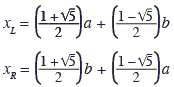
(2)	a + b = x_L + x_R
(3)
(4)
(5)	The areas of the three regions between the graphs of p(x) and L(x) are in proportion 1:2:1.

The appearance of the Golden Ratio in (1) is nothing short of surprising. Mathematician are accustomed to finding the famous constant in unexpected circumstances, but every new discovery is a delight not only for the authors but the entire community as well. (1)-(4) are of course interrelated. Below, I tackle (1)-(5) with simple algebra and polynomial integration. The simplicity of the calculations may, if not shade light on the reasons for the appearance of the Golden Ratio, at least provide a natural formal explanation for its role in the current problem.

The applet helps grasp the situation. It displays a graph of a 4^th degree polynomial whose coefficients are controlled by five sliders in the lower left corner of the applet. Each slider sports 3 draggable points: orange and red for 0 and 1, respectively. The locations of these dots define the origin and the unit of measurements for one specific axis. The blue dot then is associated with the value of a coefficient relative to the position of the origin and the unit.

This applet requires Sun's Java VM 2 which your browser may perceive as a popup. Which it is not. If you want to see the applet work, visit Sun's website at https://www.java.com/en/download/index.jsp, download and install Java VM and enjoy the applet.

What if applet does not run?

First let's see how (1) and (2) follow from (*). Since the roots of the 4^th degree polynomial p(x) - L(x) are x_L, a, b and x_R,

p(x) - L(x) = m₄(x - x_L)(x - a)(x - b)(x - x_R).

Thus the coefficients of p(x) - L(x) have the standard representation, viz.,

(**)

4:		m₄
3:		-(a + b + x_L + x_R)m₄
2:		(ab + ax_L + ax_R + bx_L + bx_R + x_Lx_R)m₄
1:		-(abx_L + abx_R + ax_Lx_R + bx_Lx_R)m₄
0:		abx_Lx_Rm₄

The comparison of coefficients by x³ in (*) and (**) shows (2). The comparison of the free coefficients (those by x⁰) shows that

(6)

x_Lx_R = -(a² - 3ab + b²).

Together (2) and (6) assert that x_L and x_R are the roots of the quadratic equation

(7)

x² - (a + b)x - (a² - 3ab + b²) = 0.

The quadratic formula applied to (7) gives (1) right away:

(1')

x_L,R = ((a + b) ± (a - b)5)/2.

(3) and (4) are easy consequences of (1'), or (1), if you will.

One additional feature that may be observed playing with the applet is that the graph of the difference p(x) - L(x) exhibits vertical symmetry. This can be easily proved from (2). Indeed, (2) implies

a - x_L = x_R - b,

which is the statement of symmetry. It can also be observed that another interpretation of (2) is the fact that the midpoints of the two intervals (a, b) and (x_L, x_R) coincide.

I claim that this is a characteristic property of the direction of the inflection line. More accurately, we have the following

Proposition

Let M(x) be a linear function. Then the graph of p(x) - M(x) has a vertical axis of symmetry iff M(x) is parallel to L(x), i.e.,

M(x) - L(x) = const.

Proof

The sufficiency (the "if" part) has been shown: (2) is a statement of the claimed symmetry. The necessity (the "only if" part) follows from the observation that all function p(x) - M(x) share the same inflection points. Indeed, the inflection points being the roots of the second derivative p''(x), do not depend on the coefficients m₁ and m₀. Or, from a different perspective, because

(p - M)''(x) = p''(x).

If there are two linear functions M₁(x) and M₂(x) such that the graphs of both differences p(x) - M₁(x) and p(x) - M₂(x) have a vertical axis of symmetry, then the inflection points of the two polynomials are those of p(x) and, hence, coincide. Therefore, as being defined by the midpoint of (a, b), the axes of symmetry of the two coincide as well. It follows that the difference

(p(x) - M₁(x)) - (p(x) - M₂(x)) = M₂(x) - M₁(x)

has the graph that is also symmetric with respect to the same vertical line. But a straight line symmetric in a vertical axis ought to be horizontal, such that necessarily

M₂(x) - M₁(x) = const.

Integration of the function p(x) - L(x) between x_L and a, between a and b, and between b and x_R immediately proves (5). In addition, because of the symmetry, the integral from (a + b)/2 = (x_L + x_R)/2 to x_R must be 0. The integration yields

(x_R - x_L)³(5(b - a)² - (x_R - x_L)²) / 240 = 0,

5(b - a)² = (x_R - x_L)²,

which is (3) in a different guise.

Remark

As we've seen, the graph of a 4^th degree polynomial that has 2 inflection points, can be symmetrized by subtracting the line through the inflection points. Here's a question for further investigation: in the absence of inflection points, can the graph of a 4^th degree polynomial be symmetrized by subtracting a linear function?

(The answer is of course, Yes. To see this, note that, whenever the second degree polynomial equation p''(x) = 0 with real coefficients has complex roots, the roots are necessarily conjugate, so that their sum and product are real numbers. Moreover, in (*), all the coefficients are real, save for the last one. The difference of two conjugate numbers is purely imaginary, so that both b - a and p(b) - p(a) are of that sort. It follows that the ratio (p(b) - p(a))/(b - a) is real. A formally constructed linear function L(x) through the (complex) points (a, p(a)) and (b, p(b)) has therefore a real slope. Its free coefficient is complex, but can be simply omitted or replaced with any real number, as its value does not affect the symmetry of the difference p(x) - L(x).)

References

L. McMullin, A. Weeks, The Golden Ratio and Fourth Degree Polynomials, On-Math Winter 2004-05, Volume 3, Number 2 (requires subscription)
L. McMullin, How I Found the Golden Ratio on my CAS, NCAAPMT newsletter, Winter 2005, 6-7.

Fibonacci Numbers

Golden Ratio in Geometry

Related material Read more...

	What Is Line?
	Functions, what are they?
	Cartesian Coordinate System
	Addition and Subtraction of Functions
	Function, Derivative and Integral
	Graph of a Polynomial of arbitrary degree
	Graph of a Polynomial Defined by Its Roots
	Lagrange Interpolation (an Interactive Gizmo)
	Equations of a Straight Line
	Taylor Series Approximation to Cosine
	Taylor Series Approximation to Cosine
	Linear Function with Coefficients in Arithmetic Progression
	Sine And Cosine Are Continuous Functions

72354367