A Plane Filling Curve for the Year 2017

J. Arioni
14 December, 2017

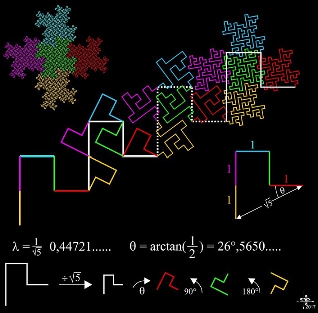
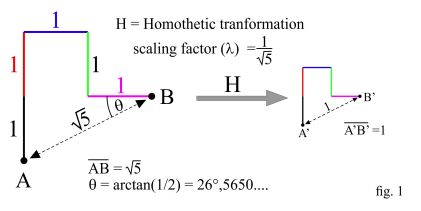
The line from A to B (A-to-B line) of fig. 1 is made up of five identical segments, whose length, for simplicity, will be assumed to be the length unit. The line from A' to B' (A'-to-B' line) is obtained by scaling the A-to-B line by a factor $\displaystyle \frac{1}{\sqrt{5}.}$

In fig. 2 five copies of the A'-to-B' line of fig. 1, differently oriented as shown in the figure, are arranged following a scheme based on their colors (starting from C: black, red, blue, green and magenta). The result is the C-to-D line.

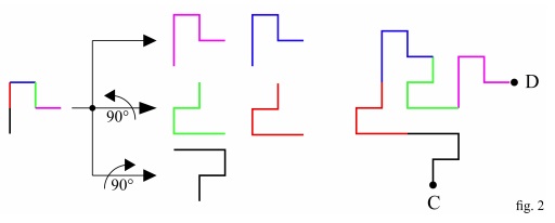
By rotating the A-to-B line of fig. 1, counterclockwise and by an angle q, we get the dashed line in the middle of fig. 3. On the right hand side of fig. 2) the dashed line has been superimposed to the C-to-D line to give an evidence that the C-to-D line can as well be obtained by substituting each segment of the A-to-B line with a scaled copy (properly oriented) of the A-to-B line itself, the factor of scaling being $\displaystyle \frac{1}{\sqrt{5}}.$

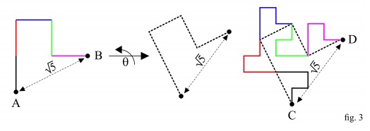
Fig. 4 shows how to get the E-to-F line (down in the figure) starting from the C-to-D line of fig. 3 and repeating (iterating) the steps described in fig. 3. Lines such as A-to-B, or C-to-D, or E-to-F will be also referred to as "curves" instead of "lines".

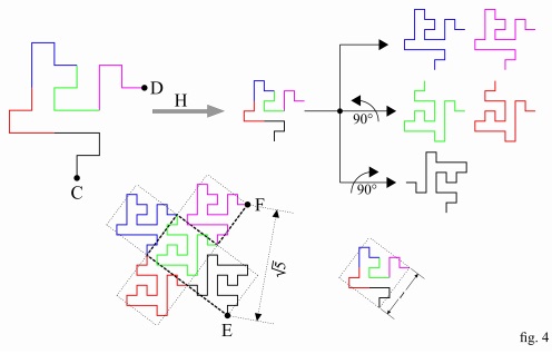
Fig. 5 shows what we get with two more iterations:

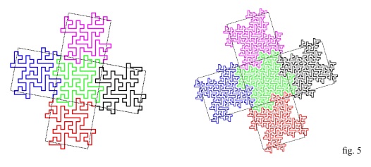
We can go on iterating the rules explained through fig 2 and fig 3 as many times as we like, with the result that the curve, step by step, will tend to fill an extremely complex geometric figure with a surface of 5 square units. Such geometric figure is roughly approximated (quite roughly indeed) by the cross formed by the five squares with dashed-line sides that are superimposed to the curves.

The squares forming the cross have sides of length $1$ (see fig. 4, bottom right), then a surface of one square unit, so that the surface of the cross is $5$ square units.

At any iteration the number of the segments that form the curve increases by a factor $5,$ while the length of any single segment decreases by a factor $\sqrt{5},$ so that the Hausdorff dimension of the curve is $\displaystyle \frac{\log(5)}{\log(\sqrt{5})} = 2,$ and that's why we can state that the curve fills a 2-dimensional figure.

Note: at any iteration, the cross superimposed to the curves rotates counterclockwise by an angle q.

Filling the Euclidean plane

In fig. 6, on the left, there are four copies of the A-to-B line of fig. 1, the first rotated by an angle $q,$ the others by an angle of $90^{\circ}$ each with respect to the former from top to bottom; the four colors are here used to highlight the orientation of the single pieces that are going to compose the curve. In the middle of the figure, copies of such lines are arranged around the spiral in black to form the curve in black on the right hand side of fig. 2. Thanks to the colors the construction should be easily intelligible.

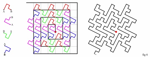
In a similar way it possible to construct the curve on the right hand of fig. 7 below (stage 2).

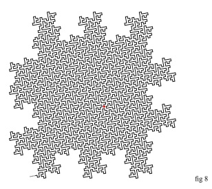
In fig. 8 below the curve as it looks after one more iteration (stage 3):

Plane Filling Curves

• Plane Filling Curves
• Plane Filling Curves: Hilbert's and Moore's
• Plane Filling Curves: Peano's and Wunderlich's
• Plane Filling Curves: all possible Peano curve
• Plane Filling Curves: the Lebesgue Curve
• Following the Hilbert Curve
• Plane Filling Curves: One of Sierpinski's Curves
• A Plane Filling Curve for the Year 2017

|Contact| |Front page| |Contents| |Did you know?|

Copyright © 1996-2018 Alexander Bogomolny