
Use of Homogeneous Coordinates for Geometric Calculations
R. F. Housholder
15 November, 2006
- Introduction
- Problem Statement
- Solution Method Discussion
- Problem Solution Examples Using In-Place Calculations
- Elementary Matrix Manipulations
- Homogeneous Coordinates
- Problem Solution Example Using Homogeneous Coordinates
- Review of Concepts
- Selected References
- C Code Examples
1. Introduction
Drawing diagrams using exact coordinate information is often required in order to accomplish certain tasks. When we draw such diagrams, it is often required that geometrical shapes within them be moved or turned in order to be correctly positioned or so that certain measurements or calculations can be made.
As an example, one might consider an electric power company which has to make sure that its transmission towers are properly oriented to support the power lines.
Also such a power company might have to comply with local ordinances requiring that any power line be some minimum distance from a tree of a certain height. If the power line twists and turns through a forested area, it can be difficult to know which trees might have to be removed.
Another example might be that you owned a piece of property that was located along side of a road. At the edge of the road, a city water pipeline is already in place. You intend to build a house on the property and would like to connect to the city water pipeline. However, there is a city ordinance that requires that you be within a certain distance of a straight section of the pipeline ends and be within some minimum tolerance distance from the pipeline.
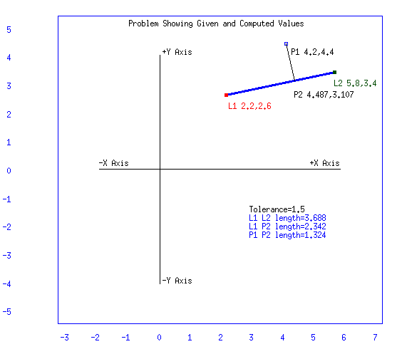
Both of these situations illustrate a problem that can be solved by geometrical methods. Basically, the requirement is that exact position and orientation information must be known. Such position information can be expressed in two dimensions, using pairs of numbers called orthogonal (right angle) coordinates. The following diagram illustrates our problem:
 | |
| Figure 1 |
Figure 1 shows information that could be, say, a power line segment from L1 to L2 and a tree located at P1. Or, just as easily, there could be a pipeline section from L1 to L2 and your house water connection could be at P1. The point here is that Figure 1 illustrates a possible real-world situation.
So now that you know that what we are about to discuss has a valid purpose and is not just a "number problem," let's state the problem in mathematical terms and go on to solve it using two methods, the latter of which, may surprise you.
2. Problem Statement
Given an arbitrary line and an arbitrary point plus some tolerance value,
What is the shortest distance between the point and the line?
Is this distance less than or equal the tolerance value?
Where is the intersection of a line from the point to the original line?
Is the point of intersection within the start and end points of the line?
3. Solution Method Discussion
There are two major methods for solving a problem such as this. The first method involves what we'll call In-Place Calculations. As the name implies, various values needed will be computed using the values given and eventually, all the unknowns will be solved.
This method involves standard geometrical techniques and requires that the slope and y-intercept of each line be computed. Then, the intersection points of the two lines can be computed.
Knowing this, the lengths of both the intersecting line and that portion of the original line up to the intersection point can then be computed, completing demonstration of the first method.
Following this, the values determined in the solution will be used to restate the problem in a manner which can easily be solved by inspection. This will be a sub-problem that still uses In-Place Calculations. However, we'll move the line so that it goes from the origin out to a location on the X axis. The point will be placed in its appropriate location and then the results will be examined.
Then, we will begin the discussion of what we need to do to use homogeneous coordinates and address the ultimate subject of this discussion. With homogeneous coordinates, we must use matrix techniques for their manipulation, so we'll backtrack a bit to see how these techniques operate. Then, we'll introduce homogeneous coordinates and show how easily they can be manipulated.
Finally, we'll show that by using techniques of homogeneous coordinates, it is possible to take our original problem as stated above, move certain values to the origin of the coordinate system, and essentially do the solution in accordance with our second, sub-problem above. The bookkeeping is greatly simplified and the method lends itself to computer implementation.
4. Problem Solution Examples Using In-Place Calculations
First, refer back to the previous diagram. We have a straight line with two endpoints and an arbitrary point not on the line. We also have a tolerance value. In the following material, each of these values plus some values that will have to be calculated as we go along are given.
The following values are given:
|
Lx1 = 2.2 Ly1 = 2.6 - Line end point #1 Lx2 = 5.8 Ly2 = 3.4 - Line end point #2 Px1 = 4.2 Py1 = 4.4 - Point T = 1.5 - Tolerance value |
The following values must be computed:
|
m1 = slope of original line b1 = Y-intercept value of the original line m2 = slope of connecting line b2 = Y-intercept value of the connecting line Px2 and Py2 are the intersection point coordinates of the original and the connecting lines Ln1 = Length of original line Ln2 = Length of connecting line Ln3 = Length of original line up to the intersection point |
The slope, m1, and Y-intercept, b1, of the original line are calculated:
|
Next, we rely on the fact that an orthogonal line is the shortest distance from a point to a line and that the slopes of orthogonal lines are the negative reciprocals of each other, as long as neither one is zero. Therefore, the slope of the intersecting line is:
|
Using the two slopes and Y-intercept formulas, a simultaneous equation can be set up and solved for one of the coordinates. We have two equations and two unknowns. Let's choose the y intersecting point, Py2:
|
Py2 = 0.222 Px2 + 2.111 Py2 = -4.505 Px2 + 23.321. |
Setting the above two equations so they equal each other and solving for Px2 gives:
|
0.222 Px2 + 2.111 = -4.505 Px2 + 23.321 0.222 Px2 + 4.505 Px2 = 23.321 - 2.111 4.727 Px2 = 21.21 Px2 = 21.21 / 4.727 = 4.487. |
Py2 can now be obtained by substituting the value of Px2 into either line equation; this gives:
|
The intersecting line length can be calculated using the Pythagorean theorem:
|
In order to verify whether or not the intersection point falls within the ends of the line, we must calculate the length of the line and the length from the leftmost end of the line up to the intersection point.
Again, using the Pythagorean formula, the length of the original line is:
|
And, the length of the line up to the intersection point on the original line is:
|
Now, we have all the information required to evaluate point P1:
Length Ln2 is less than the tolerance value:
|
Ln2 = 1.324 T = 1.5 1.324 is < 1.5 |
and length Ln3 is less than Length Ln1:
|
Ln3 = 2.342 Ln1 = 3.688 2.342 is < 3.688 |
This may seem like a lot of work and, in some respects, it is. Part of the difficulty is in the bookkeeping necessary to keep everything "straight." Imagine the difficulty if one had to compute the above calculations for hundreds or thousands of points.
As stated in the second of the solution methods in Section 3, above, there is a situation whereby the calculations are reduced considerably. Let's assume that we had a line that started at the origin and went out on the X axis to the coordinates 3.688, 0.0. Let's further assume that we had a point located at 2.342, 1.324 and that the tolerance of 1.5 was still in effect. Figure 2 shows this configuration:
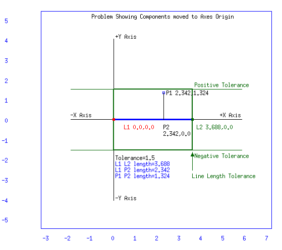 | |
| Figure 2 |
This problem is instantly solvable by examination:
|
Lx1 = 0.0 Ly1 = 0.0 Lx2 = 3.688 Ly2 = 0.0 Px1 = 2.342 Py1 = 1.342 T = 1.5 |
All the information we need in order to solve the problem is already present and no calculations have to be performed except to compare the existing values. The line, L1 is coincident with the X axis, therefore, the distance to it from point P1 is simply the y coordinate value of Py1. The intersection point's X coordinate is simply the value of Px1. Therefore, the length of line L1 up to the intersection point is the same value. Comparisons can be made with the tolerance value and the total length of line L1 quite easily.
In fact, a green tolerance box has been drawn to emphasize this. If the point, P1 is in the box, then its location meets the tolerance constraints.
The point of this second example solution was to show that the difficulty of a problem can often be considerably reduced by choosing the position and location where such comparisons are to be performed. Note that the values used in this second problem were derived from the answers from the first problem.
The last possibility given in Section 3, above was to convert coordinates so that the situation just discussed could be created. It turns out that by using homogeneous coordinate techniques, this transformation can be easily performed.
And so, we have finally reached the point in our discussion where the key reason for all of our work comparing two ways to do the same thing can be stated and it is this:
| In certain geometrical problems, it is often easier to move the data before measurements are made. This, of course requires that we have some method which can be used to do the moving of the geometrical coordinates. The technique used to do this is the subject of the rest of this discussion, namely, Homogeneous Coordinates. |
Before we can discuss them, however, we need to cover the basics of the techniques required to manipulate them. These techniques involve the use of matrix arithmetic and will be discussed next.
After that, we will show how simple our problem can be made by using these techniques. Of special importance is the bookkeeping associated with such a problem. We now have the motivation for continuing our discussion.
5. Elementary Matrix Manipulations
In the following material, we will limit our discussion to only those aspects of matrix manipulation that are necessary for our specific task. Interested readers should consult other sources for material not covered below.
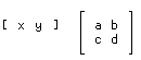
A matrix is simply a significant ordered rectangular array of numbers (elements). Matrices are sometimes written so that the elements are enclosed within left and right bracket symbols:
 |
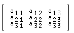
The elements that make up a matrix are often denoted by a row and column subscript:
 |
Mathematical operations can be performed on matrices and these operations follow certain rules. We will be concerned primarily with multiplication, but it is instructive to show how addition and subtraction are handled. These two matrix operations are handled on a one-for-one element basis. For example, the following diagram is an example of two, 3 x 3 matrices being added:
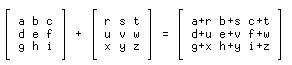 |
Note that the resulting, solution matrix contains elements that are the sums, on a one-for-one basis, of the elements in the two matrices that are being added together.
Matrix multiplication is handled slightly differently and will be the focus of subsequent material. Examine the following diagram:
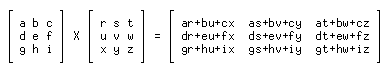 |
Here, each final element is the result of the summation of three element-multiplication operations. However, a bit of analysis is required. Note that all the members of the top row of the first matrix (a, b, and c) appear in the top ROW of the result matrix.
However, all the members of the top row of the second matrix (r, s and t) appear in the leftmost COLUMNS of the resultant element sums. While the first matrix uses a column-within-row traversal, the second matrix uses a row-within-column traversal.
Another difference between matrix addition and matrix multiplication has to do with the sizes of the matrices. In addition, both matrices must be the same size: that is, the number of rows of the first matrix must equal the number of rows in the second. The same is true for the number of columns.
In matrix multiplication, two matrices can be multiplied as long as they share at least one common dimension: either they must have the same number of columns or the same number of rows.
As we have just shown, they can also have the same number of columns and rows. For example, if we wanted to multiply a 1-row, 3-column matrix by a 3-row, 3-column one, the result would be as shown in the next diagram:
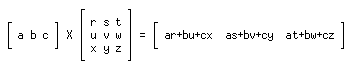 | |
| Figure 3 |
Note that the answer is only the first row of the answer shown in the previous diagram.
There is an example that we will use later that has some important qualities. It is called an identity matrix. An identity matrix is constructed so that all matrix locations contain zeros except for the top-left to bottom-right diagonal. Those positions contain ones. Consult the following diagram:
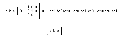 |
As can be seen, when the first matrix is multiplied by the identity matrix, there is no change in the result:
| [ a b c ] = [ a b c ] |
The concept of the identity matrix will be referenced in the following material.
These matrix manipulation rules are all we will need in order to use matrix techniques to help simplify the problem of performing transforms on coordinates. Before we get into those details, however, we must digress a bit further and cover the use of Homogeneous Coordinates.
6. Homogeneous Coordinates
Homogeneous coordinates are a technique for simplifying mathematical operations on coordinates by increasing their dimensionality. Again, we are only going to cover those aspects of homogeneous coordinates that will be required for our purpose. Interested readers are urged to consult appropriate references to obtain more information on additional aspects of homogeneous coordinate operations.
Homogeneous coordinates can be expressed as matrices. The reference to increasing their dimensionality means that 2-dimensional coordinates are converted to 3-dimensions by the addition of a scaling factor as the third coordinate.
Fortunately, in our implementation, this scaling factor is always equal to 1.0. For example, let's say that we had a location that was expressed by the coordinates 'x' and 'y'. In homogeneous form, they would look like this:
| [ x y 1.0 ] |
Or sometimes like this:
| [ x y 1 ] |
The ending 1.0 is a value that must be present so that certain matrix manipulation operations will work correctly but, as we shall see, is not used after the value of the resultant transformation has been calculated.
Returning to our ultimate problem: we were given two arbitrary line end point coordinates and it our desire to move the line so that one point is on the origin and the other extends out on the x axis. How can this be done?
Answer: by performing transforms on the original coordinates. Specifically, we must perform a translation (linear movement) on both end points such that one of them is coincident with the origin. Then, we must perform a rotation of the line so that the point that was not moved to the origin is located on the X axis.
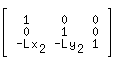
So our first task is to express this pair of coordinate transforms in matrix format. Two-dimensional transform representation in homogeneous coordinate format requires a three-dimensional matrix: one that is 3 rows by 3 columns. Starting with an identity matrix, a transform matrix that will move the point Lx1, Ly1 to the origin is:
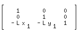 |
If we were to convert the coordinates for Lx1, Ly1 into homogeneous form, we would simply add the extra position and make the 1 x 3 matrix:
| [ Lx1 Ly1 1 ] |
Look what happens when we multiply these two matrices:
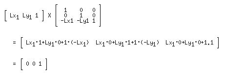 |
The resultant x value is 0 and the resultant y value is 0. (Remember, we said that the final 1 wasn't needed any more after the calculation has taken place?) What this means is that the first matrix held the values of the coordinates of the point L1. The second matrix contained the translate transform that converted the point L1 to be at 0.0, 0.0: the origin.
The interesting thing is that this same translate transform matrix could be used to translate any point by the amount -Lx1, -Ly1. In fact, if we apply the same transform to the point Lx2, Ly2, we'd end up with the two line endpoints in exactly the same relationship to each other as they were originally, but they would be translated so that L1 was at the origin. The angle that the line makes with the X axis and the length of the line would be unchanged.
The following link shows the result of applying the translation matrix to our original data: the arbitrary line and the associated arbitrary point. Here, both endpoints of the line and the arbitrary point are all processed by the translate transform using the matrix techniques just discussed.
Please note that this animation shows how the movement is performed. It is intended to show that the line and the point are all simply moved in a linear manner so that the first line end point, L1 rests on the origin.
In reality, the transformation is instantaneous and does not slowly move the data as shown in the animation. The slower movement is done in order to emphasize the relationships of the data being moved: only translation takes place.
|
Link to Animated Sequence showing Translate Transform |
However, we're not finished, because after translating both line endpoints, we still have to rotate the line down so that it is coincident with the X axis. We need to construct a rotation transform that can be applied to the line endpoints. Then, this transform must be expressed in matrix format using homogeneous coordinates and a matrix multiplication operation needs to be carried out to actually perform the rotation.
First, some words on rotation transforms: Rotation occurs only around the coordinate axes. That does not mean that we can't rotate some geometrical shape about an arbitrary point. It just means that, from a mathematical sense, the rotation would be performed using the following steps:
Select the location of the center of rotation.
Translate everything such that the negative, in both X and Y, of the chosen center of rotation is subtracted from every coordinate pair.
Perform the rotation transform (to be described next).
Translate everything back by adding the original center of rotation to each coordinate pair.
In our case, however, only the first three steps will be performed because our objective is to transform the points to a location where it is easier to make certain measurements. So, we continue with our discussion on rotation transforms.
A rotation transform is based on an angle. The angle can be defined in terms of the ratios of the sides of a triangle defining the points to be rotated. In our case, a triangle can be defined such that the y component is the difference in the y coordinate values. Specifically:
|
Ly2 = 3.4 and Ly1 = 2.6 |
Subtracting the values gives: 3.4 - 2.6 = 0.8. Similarly, the same thing is done for the x component:
|
Lx2 = 5.8 and Lx1 = 2.2 |
subtracting the values gives: 5.8 - 2.2 = 3.6.
These two values, 0.8 and 3.6 can be used to calculate a ratio that is equivalent to the tangent of the angle, theta, for which we are seeking.
Performing the division gives a tangent theta value of: 0.8 / 3.6 = 0.22222.
So, the angle is the angle whose tangent is 0.22222 or 12.53 degrees. In mathematical terms, this value is called the arctangent of 0.22222. The angle could also be expressed as 0.2187 radians.
The rotation transform needs two values: a sine and a cosine of the angle of rotation. Now that we have the angle, it is a simple matter to obtain the sine and the cosine:
|
sinθ = sin 0.2187 = 0.2169 cosθ = cos 0.2187 = 0.9762 |
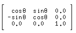
The rotation transform, expressed for a positive-going angle (one that is clockwise) is defined as follows:
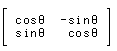 | |
| Figure 4 |
Since our rotation will be in the positive direction (i.e. clockwise), the matrix will be in the above form.
Recall that the rotation transform must be placed into homogeneous coordinate form. All that means is that an extra row and column must be added to the matrix just shown. We simply start with an identity matrix and place the 2×2 matrix pattern shown in Figure 4, in the upper left corner of the 3×3, identity matrix:
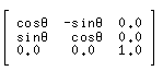 |
If the first coordinate of our line, the one that is now at 0.0 is put into homogeneous form and multiplied by the above rotation matrix, there will obviously be no change because the coordinates of that point are now 0.0, 0.0. The homogeneous form of this point will, therefore be:
| [ 0.0 0.0 1.0] |
Using the matrix multiply procedure, one can see that everything in the above matrices except the final 1.0 will be zero.
However, the second point will be rotated by exactly the required amount to make its y component 0.0 and it's x component the length of the line.
Using the template shown above in Figure 3, we can make an example computation for the point L2, which has now been moved by the translate transform. As we just calculated:
| Lx2=3.6 and Ly2=0.8 |
If we plug in these values for the coordinate matrix and the appropriate sine and cosine values for the rotation transform matrix, we will obtain the result shown in the next figure:
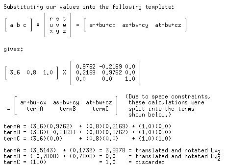 |
Checking the values of Lx2 and Ly2, we do, in fact have the the same values that we calculated previously above. The x coordinate is the line length and the y coordinate is zero. The following link shows the effect of applying the rotation transform to the points resulting from application of the translation transform.
Recall that in the animation sequences, a smooth motion is shown when, in reality, the rotation matrix sends the transformed points directly to their new locations.
This animation is intended to show that the rotation is applied to both the line and the point in proper proportion. The rotation takes place around the origin and, since point L1 occupies that location, the rotation transform has no effect on that point.
|
Link to Animated Sequence showing Rotation Transform |
The problem is that it took us two, distinct operations to achieve this result. First, we had to construct a transform to translate the coordinates to the origin, relative to the first point in the line. Next, we had to construct a transform to rotate the points around the axis origin.
The somewhat surprising solution to this problem, however, is that there is a way to combine the two coordinate transforms into a single one, that performs both actions: translation followed by rotation. The process of combining transforms is called concatenation and, if each transform is expressed in matrix form, the combination is performed by matrix multiplication.
Since we have covered the format of both the translation and the rotation transforms and their expression in homogeneous matrix format, the following figure probably does not need too much additional explanation. In it, one can follow the order of translation and rotation matrix element access in each of the two matrices. Remember that the first matrix is accessed by column within row and the second is row within column.
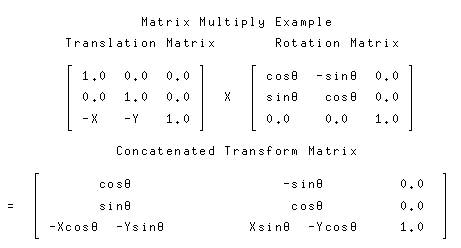 | |
| Figure 5 |
In order to help visualize the matrix multiplication procedure that makes the concatenated transforms, the following link shows an animated version of the steps needed to obtain the matrix shown in Figure 5.
|
Link to Animated Sequence showing Matrix Multiply Operation |
The animation above shows how the two matrices can be combined using the rules for such combination. One consideration we must take into account, though, is that the ORDER in which the matrix multiplication takes place is important.
In our case, the Translation matrix must be first and the Rotation matrix second. This is because, matrix multiplication is not commutative. The order in which the matrices are multiplied is important.
Once the combined transform matrix has been created, our original line can be transformed to the origin and along the X axis. Additionally, ANY other point in our original diagram can be modified by the same transform so that its coordinates are in the same relationship as the original point was to the original line.
7. Problem Solution Example Using Homogeneous Coordinates
With the concatenation of the Translate and Rotate transforms, we now have the ability to do what we set out to do, namely: to convert the DATA into a form where our desired tolerance measurements can be applied without having to go through all of the calculations we used with the In-Place Calculation method covered in section 4.
The next link shows the result of our efforts and illustrates the effect of applying the concatenated matrix above to the original data points. Again, this animation uses a movement that shows the gradual translation and rotation. In reality, of course, the transformation is instantaneous.
|
Link to Animated Sequence showing Use of the Concatenated Transform |
So, one can easily see that the second version of our original problem can be achieved by constructing a combined transform matrix to first move everything into a format where the needed comparisons can be performed.
Now that we have a better understanding of the value of using homogeneous coordinates and homogeneous coordinate transforms, let's use them to quickly check the effect of choosing the opposite end of our original line as the one that is moved to the origin.
Take a look at the following link.
|
Link to Animated Sequence showing Use of Other End of Line |
Here, the opposite end of the line, L2, was used as the point that was moved to the origin. Again, in the above link, the motion is for illustrative purposes only, since the homogeneous transform instantly converts the appropriate points to their final locations. Refer again to Figure 1 and the coordinates for L2. Here, the translate matrix will have to be the negative of L2's coordinates in order to move L2 to the origin:
 |
The rotation matrix also has to be constructed with angles defined from L2. The x and y differences have to be of opposite sign. Before, we had values of
| x difference of 3.6 and y difference of 0.8. |
Since we are going in the opposite direction from a different vertex of the defining triangle, the sine, cosine and angle, θ, as well as its tangent are defined differently:
| x difference of -3.6 and y difference of -0.8. |
These values produce an arctangent of -3.6/-0.8 for a theta of 77.47 degrees or 1.352 radians. Note, since the rotation is from point L2, that in order to get into alignment with the X axis, the angle is measured in the counter-clockwise direction, which is opposite from the rotation direction when L1 was used. If we plug in these values for the appropriate sine and cosine values, we obtain the following rotation transform matrix:
 |
These two transforms, in matrix representation, are concatenated by using the matrix multiplication procedure shown above and the result is used to convert L1, L2, and P1. Note that, since L2 was chosen, the sense of the directions is changed and point P1 ends up with a negative Y value. However the important point to note is this:
| THE RELATIVE POSITIONS OF ALL POINTS ARE MAINTAINED REGARDLESS OF THE END OF THE LINE THAT WAS CHOSEN TO BE MOVED. |
This also explains why the tolerance was expressed in both positive and negative Y values.
8. Review of Concepts
So, we come to the end of our discussion regarding homogeneous coordinates and their use in manipulating geometrical values. The main points of the discussion are:
Sometimes it is easier to move the data to a position where measurements can be made rather than make the measurements or calculations in place.
Homogeneous coordinates allow the creation of transforms that can be combined to perform complex operations on a large number of locations.
These transforms can be expressed as matrices and their use follows standard matrix manipulation principles.
Often, the bookkeeping required to manipulate a large number of coordinates is greatly reduced by using homogeneous coordinates and matrix manipulation techniques to combine all of the operations required so that a much smaller, overall computational effort is required.
9. Selected References
The author used information contained in several texts for some of the information used in the above presentation as well as various references available on the Internet. Listed below are some of the references used:
- William M. Newman and Robert F. Sproull, Principles of Interactive Computer Graphics, Second Edition, International Student Edition, 1979, McGraw-Hill
- David F. Rogers and J. Alan Adams, Mathematical Elements for Computer Graphics, Second Edition, 1990, McGraw-Hill
- Howard Eves, Elementary Matrix Theory, 1966, Dover Publications
- Lloyd L. Smail, Analytic Geometry and Calculus, Appleton-Century-Crofts, Inc.
- James Stewart, Calculus, 1995, Brooks/Cole Publishing Company
10. C Code Examples
The above article is intended primarily for those individuals who are learning about homogeneous coordinate transforms. Therefore, the emphasis has been on principles and not on implementation in any specific computer language. However, there may be, among the readers, certain individuals who would like to see the implementation of some of the principles in specific computer code.
Therefore, two very short subroutines in the C computer language are offered. One important aspect of these examples is that they emphasize the idea that was briefly discussed in the above material and that is the idea of simplifying the bookkeeping involved in the mathematics of coordinate manipulation. These two routines show how simple it is to realize some of the ideas expressed above in specific programming implementations.
concatenateMatrix.c is a routine that can be called to perform matrix multiplication on 3×3 matrices, defined as double[3][3].
void concatenateMatrix(double M[3][3],double N[3][3],double C[3][3])
  {

  /* this routine concatenates two input transforms in matrix format,
  -  M and N, and places the result in matrix C */
  int j;
  int i;
  int k;

  for(j=0;j<3;j++)
    {
    for(i=0;i<3;i++)
      {
      C[j][i]=0.0;
      for(k=0;k<3;k++)
        C[j][i]+=M[j][k]*N[k][i];
      }
    }
  }
multiplyMatrix.c is a routine that multiplies a homogeneous position vector (a point that is expressed in homogeneous coordinates as a 1×3 matrix) by a 3×3 matrix.
void multiplyMatrix(double I[3],double C[3][3],double T[3])
  {

  /* this routine performs a matrix multiply of the input, 1-D matrix I
  -  with the 2-D matrix C and places the result in matrix T.
  -  NOTE that the last term of the T matrix (the '1.0' does not
  -  need to be computed */

  T[0]=I[0]*C[0][0]+I[1]*C[1][0]+C[2][0];
  T[1]=I[0]*C[0][1]+I[1]*C[1][1]+C[2][1];
  }
|Front page| |Contents| |Geometry|
Copyright © 1996-2018 Alexander Bogomolny74390698