Recipes for the "Average Value" of a function.

Scott E. Brodie
5/18/99
 
 

Most everyone is familiar with the procedure for taking the average of a (finite) collection of numbers. You add up the values, and divide by the number of terms in the sum:

.

Sometimes, the list of number values is purely empirical (say, the heights of the children in a third grade classroom), and little more can be said about the averaging process. However, the list of numbers often arises as the set of values of some known function, evaluated at each point on a list of values of the function argument:

.

For example, one might record the temperature once every hour ("on the hour"), and then compute the average temperature over the course of a day or a month.

In many cases, the values x_j of the function argument are of little interest in themselves. For example, one might be interested in the hourly temperatures in order to estimate the cost of air-conditioning one’s bedroom over the course of the summer. In a case such as this, one expects the hourly temperatures to vary only slowly from one hour to the next, so that the average temperature for a particular day would be about the same whether one recorded the temperatures "on the hour" or "on the half-hour". In such a case, it is convenient to think of the average as a property of the function (and the interval over which it is averaged), rather than as a property of the set of sampling points.

Occasionally, the temperature might change unusually rapidly. In order that the average not be misleading, in such an instance, it would be necessary to measure the temperature more frequently, say, once every 5 minutes. This would allow the record of temperatures to reflect a much briefer "spike" or "step". The contribution to the average from the hours when the temperature changes but little would not be altered by the increased sampling frequency, as the greater number of values incorporated into the sum for the average would just be counterbalanced by the division step, where we would divide by a proportionately greater count.

In general, the procedure works like this: suppose we wish to average a function f over a closed, finite, interval [a, b]. Divide up the interval [a, b] into n equal sub-intervals, I_j each of length (b – a) / n. For each interval I_j, choose , and form the average

The average obtained in this way will depend, in principle, on the particular choice of the x_j’s. However, if the function f is sufficiently "smooth", this dependence on the particular x_j’s will be slight, particularly for large n. In the most favorable cases, the limit

     (*)

may exist no matter which x_j’s are chosen. In these favorable cases, the limit (*) defines "the average of f over the interval [a, b]."

It is one of the major goals of a traditional basic course in Calculus to show that the limit (*) exists whenever f is continuous on the interval [a, b]. However, the limit (*) may exist even for functions which fail to be continuous over any interval, so the condition of continuity, while "sufficient," is not "necessary" for the average (*) to exist.

It is instructive to look at this formula from two additional points of view: denote the common length of the subintervals I_j by Dx. Then we have

Dx = (b - a) / n, or
 

Dx/(b - a) = 1/n
 
 

Substituting in (*) gives

But f(x_j)·Dx is the area of a small rectangle whose height is f(x_j) and whose width is Dx, and  is just the area bounded by the x-axis, the vertical lines

x = a, x = b,

and the graph of the function f. In other words, the average of f over the interval [a, b] is the height of a rectangle whose base is the interval [a, b] and whose area is the same as that under the graph of f.

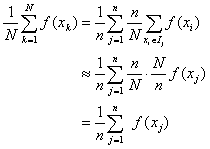
Now suppose that, instead of deliberately choosing points, one each, from the equal subintervals I_j of [a, b], we choose the points x_k from the interval [a, b] at random. Suppose we choose a total of N points. We can still use the n equal subintervals I_j to keep track of the distribution of the points x_k. In the long run, the contribution of each subinterval to the sample will approach will contribute N / n points. (This is essentially what is meant by saying that the points have been chosen "at random".) If the subintervals I_j are small enough (and the function f smooth enough), we can pick a single representative value, say x_j, for each subinterval, and approximate the average as follows:

Evidently, the random sampling process yields the same average as we obtained previously by picking exactly one point from each subinterval.

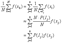
If we wish to allow for the possibility that some x_i values are more likely than others, only a slight adjustment is necessary. Just denote by P(I_j) the probability that a randomly chosen x_i falls in the interval I_j. In the long run, the subinterval I_j will contribute N· P(I_j) terms to the average. In this case,

Thus, the limit of a sum of the form  can be interpreted as an average of the function f. Of course the value of the average may depend on the choice of the probability distribution P as well as the function f. In the case where the probabilities are proportional to the lengths of the intervals I_j – that is, where the distribution is "uniform", this kind of average agrees with the usual one.